Tutorial (Optimization Toolbox)

Optimization Toolbox

Nonlinear Equations with Analytic Jacobian

This example demonstrates the use of the default medium-scale fsolve algorithm. It is intended for problems where

The system of nonlinear equations is square, i.e., the number of equations equals the number of unknowns.
There exists a solution such that .

The example uses fsolve to obtain the minimum of the banana (or Rosenbrock) function by deriving and then solving an equivalent system of nonlinear equations. The Rosenbrock function, which has a minimum at , is a common test problem in optimization. It has a high degree of nonlinearity and converges extremely slowly if you try to use steepest descent type methods. It is given by

First generalize this function to an n-dimensional function, for any positive, even value of n:

This function is referred to as the generalized Rosenbrock function. It consists of n squared terms involving n unknowns.

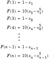
Before you can use fsolve to find the values of such that , i.e., obtain the minimum of the generalized Rosenbrock function, you must rewrite the function as the following equivalent system of nonlinear equations:

This system is square, and you can use fsolve to solve it. As the example demonstrates, this system has a unique solution given by .

Step 1: Write an M-file bananaobj.m to compute the objective function values and the Jacobian.

function [F,J] = bananaobj(x);
% Evaluate the vector function and the Jacobian matrix for 
% the system of nonlinear equations derived from the general 
% n-dimensional Rosenbrock function.
% Get the problem size
n = length(x);  
if n == 0, error('Input vector, x, is empty.'); end
if mod(n,2) ~= 0, 
   error('Input vector, x, must have an even number of 
components.'); 
end
% Evaluate the vector function
odds  = 1:2:n;
evens = 2:2:n;
F = zeros(n,1);
F(odds,1)  = 1-x(odds);
F(evens,1) = 10.*(x(evens)-x(odds).^2); 
% Evaluate the Jacobian matrix if nargout > 1
if nargout > 1
   c = -ones(n/2,1);    C = sparse(odds,odds,c,n,n);
   d = 10*ones(n/2,1);  D = sparse(evens,evens,d,n,n);
   e = -20.*x(odds);    E = sparse(evens,odds,e,n,n);
   J = C + D + E;
end

Step 2: Call the solve routine for the system of equations.

n = 64;  
x0(1:n,1) = -1.9; 
x0(2:2:n,1) = 2;
options=optimset('Display','iter','Jacobian','on');
[x,F,exitflag,output,JAC] = fsolve(@bananaobj,x0,options);

Use the starting point for the odd indices, and for the even indices. Accept the fsolve default 'off' for the LargeScale parameter, and the default medium-scale nonlinear equation algorithm 'dogleg'. Then set Jacobian to 'on' to use the Jacobian defined in bananaobj.m . The fsolve function generates the following output:

                                Norm of  First-order Trust-region
Iteration Func-count   f(x)        step   optimality       radius
    0        1      4281.92                    615            1
    1        2      1546.86           1        329            1
    2        3      112.552         2.5       34.8          2.5
    3        4       106.24        6.25       34.1         6.25
    4        5       106.24        6.25       34.1         6.25
    5        6      51.3854      1.5625       6.39         1.56
    6        7      51.3854     3.90625       6.39         3.91
    7        8      43.8722    0.976562       2.19        0.977
    8        9      37.0713     2.44141       6.27         2.44
    9       10      37.0713     2.44141       6.27         2.44
   10       11      26.2485    0.610352       1.52         0.61
   11       12      20.6649     1.52588       4.63         1.53
   12       13      17.2558     1.52588       6.97         1.53
   13       14      8.48582     1.52588       4.69         1.53
   14       15      4.08398     1.52588       3.77         1.53
   15       16      1.77589     1.52588       3.56         1.53
   16       17     0.692381     1.52588       3.31         1.53
   17       18     0.109777     1.16206       1.66         1.53
   18       19            0   0.0468565          0         1.53
Optimization terminated successfully:
 First-order optimality is less than options.TolFun

Additional Arguments: Avoiding Global Variables Nonlinear Equations with Finite-Difference Jacobian