

| Nonlinear Control Design Blockset | |
Optimization Algorithmic Details
As mentioned in the Tutorial, the Nonlinear Control Design Blockset transforms the constraints and simulated system output into an optimization problem of the form
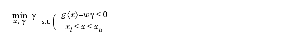
where the boldface characters denote vectors. This type of optimization problem is solved in the Optimization Toolbox routine constr. In reference to the last section,
The Sequential Quadratic Programming (SQP) method used by constr solves a Quadratic Programming (QP) problem at each iteration and updates an estimate of the Hessian of the Lagrangian. The line search is performed using a merit function. The routine uses an active set strategy for solving the QP subproblem.
The implementation of the SQP subproblem attempts to satisfy the Kuhn-Tucker equations, which are necessary conditions for optimality of a constrained optimization problem. The principal idea of the SQP algorithm forms a QP problem at each iteration based on the quadratic approximation of the Lagrangian function.
The QP solution procedure involves two phases: the first phase involves the calculation of a feasible point (if one exists); the second phase involves the generation of an iterative sequence of feasible points, which converge to the solution. In this method, an active set is maintained of the active constraints at the solution point. Virtually all QP algorithms are active set methods. This point is emphasized because many different methods exist, which are very similar in structure but which are described in widely different terms.
The routine constr further exploits the special structure of the constrained problem. For example, it can be shown from the Kuhn-Tucker equations that the approximation to the Hessian of the Lagrangian, should have zeros in the rows and columns associated with the variable  . However, this results in only a positive semi-definite Hessian which requires a more elaborate (slow) QP solution technique. Instead the algorithm initializes the Hessian matrix with ones along its diagonal except for the element associated with , which is initialized to a small positive number (e.g., 1e-10). Throughout the optimization, the code maintains zeros in all rows and columns of the Hessian associated with except the diagonal element, which is maintained at the small number. This allows the code to use a fast converging positive definite QP method while at the same time exploiting the problem's special structure.
The routine constr relates the status of the QP algorithm in the last column of the display output (the column labeled Procedures). Generally no display appears in the column meaning the Hessian is positive definite. For nonpositive definite Hessians, two successive modifications can be performed to make the Hessian positive definite. If the first modification succeeds, the message mod Hess appears in the Procedures column. The second modification always results in a positive definite Hessian and displays mod Hess(2) in the Procedures column. Often such messages imply that the optimization is far from a solution or that the problem is particularly sensitive to variations in some of the tunable parameters.
A nonlinearly constrained problem can often be solved in fewer iterations using SQP than an unconstrained problem. One of the reasons for this is that, due to the limits on the feasible area, the optimizer can make well informed decisions regarding directions of search and step length. This characteristic of the nonlinearly constrained problem is advantageous to the Nonlinear Control Design Blockset problem formulated since calculation of the cost function is computationally time consuming (it requires simulation of the system). Time saved due to fewer iterations more than compensates for the additional overhead associated with the constrained formulation.
For more information on the algorithms discussed in this section, see the Optimization Toolbox documentation.
| | Problem Formulation Details | Representation of Time-Domain Constraints | |