Mapping Toolbox

Regular Matrix Maps

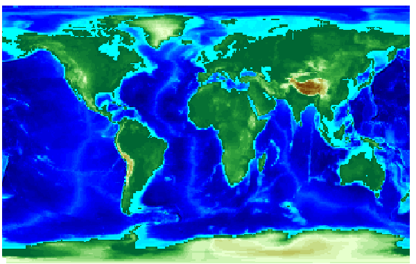
A regular matrix map is one in which columns of data run south to north, rows of data run west to east, and each matrix element represents the same angular step in each direction, for all rows and columns. For example, if each row represents one degree of latitude, and each column one degree of longitude, and the matrix is aligned north and south, then it is a regular matrix map. The topo map provided with MATLAB is such a regular matrix map.

The Map Legend

Many regular matrix maps do not cover the entire planet. It is therefore necessary to identify the scale and placement of the map with a special data structure, the map legend. The map legend is a three-element vector that identifies the size of each matrix entry and the coordinates on the globe of the northwestern corner of the map. The three entries are given in terms of angular units of degrees only. The specific format of the structure is as follows:

• maplegend = [cells/angleunit north-latitude west-longitude]
  

For the topo matrix map, each matrix cell represents one degree, the northern edge is the North Pole, and the western edge is the Prime Meridian. Therefore, the map legend for topo is

• topolegend = [1 90 0]
  

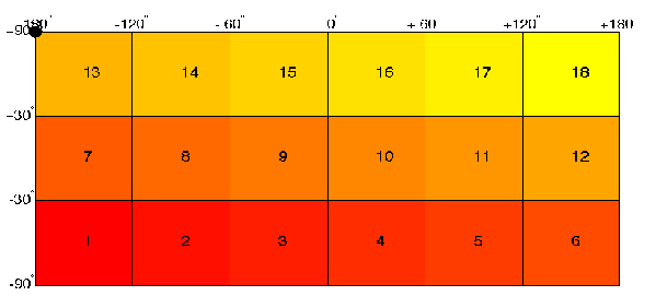
This map legend structure is stored in the topo workspace. Imagine an extremely coarse map of the world in which each cell represents 60°. Such a map matrix would be 3-by-6, and its map legend would be

• maplegend = [1/60 90 -180] = [0.0167 90 -180]
  

In this case, the map's western edge is the International Date Line, at 180°W:

Note that the first row of the matrix is displayed as the bottom of the map, while the last row is displayed as the top. All regular matrix maps in the Mapping Toolbox, as well as regular surfaces in MATLAB, are displayed in this fashion.

As an example of a matrix map that does not encompass the entire world, load the Cape Cod image using the loadcape script:

• loadcape
  maplegend
  maplegend =
      120    44   -72
  

The maplegend indicates that there are 120 cells per angular degree. This has a horizontal resolution 120 times finer than that of the topo matrix map, which was one cell per degree. The cape region covered here extends from 41°N to 44°N, and from 72°W to 69°W:

• [latlimits,longlimits] = limitm(map,maplegend)
  latlimits =
      41    44
  longlimits =
      -72   -69
  

The Geographic Meaning

A matrix map and its associated map legend can provide a host of geographic information regarding the map and its entries. First, as was just demonstrated, the north, south, east, and west limits of the mapped area can be determined as follows:

• load russia
  [latlim,longlim] = limitm(map,maplegend)
  latlim =
      35    80
  longlim =
      15   190
  

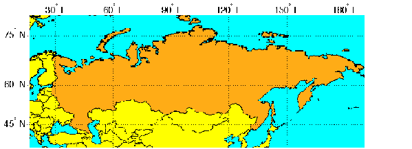
The map in the russia workspace extends over the International Date Line (180° longitude). You could use the previously described command npi2pi to rename the eastern limit to be -170, or 170°W.

The command setltln allows you to determine the geographic coordinates of a particular matrix element. The returned coordinates actually show the center of the geographic area represented by the matrix entry:

• row = 23; col = 79;
  [lat,long] = setltln(map,maplegend,row,col)
  lat =
      39.5000
  long =
      30.7000
  

You can also determine the row and column of the matrix map entry containing a given point:

• [r,c] = setpostn(map,maplegend,lat,long)
  r =
      23
  c =
      79
  

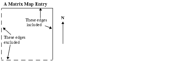
Each matrix entry can be thought of as an angular square which includes its northern and eastern edges, but not its western and southern edges.

The exceptions to this are that the southernmost row (row 1) also contains its southern edge, and the westernmost column (column 1) contains its western edge, except when the map encompasses the entire 360° of longitude. In that case, the westernmost edge of the first column is not included, because it is identical to the easternmost edge of the last column. These exceptions ensure that all points on the globe can be represented exactly once in a regular matrix map.

Although each map matrix entry represents an area, not a point, it is often convenient to assign singular coordinates for reference. An entry is defined by the point in the center of the area represented by the entry. For example, reference the center cell coordinate for the 3rd row, 17th column, of the Russia map:

• row = 3; col = 17;
  [lat,long] = setltln(map,maplegend,row,col)
  lat =
      35.5000
  long =
      18.3000
  

Since the cells in the Russia matrix map represent 0.2° squares (5 cells per degree), the cell in question extends from 35.6°S to 35.4°S and from 18.2°E to 18.4°E.

Accessing Matrix Map Elements

The actual values contained within the map matrix entries are important as well. The Mapping Toolbox provides several functions for accessing and altering the values of matrix map entries.

If the actual row and column of a desired entry are known, then a simple matrix index can return the appropriate value. Use the row and column from the last example (3rd row, 17th column) to determine the value of that cell:

• value = map(row,col)
  value =
      2
  

More often, the geographic coordinates are known:

• value = ltln2val(map,maplegend,lat,long)
  value =
      2
  

The latitude-longitude coordinates associated with particular values in a matrix map can be found with findm, which is similar to the standard MATLAB command find. Here we find the coordinates in the topo map with values greater than 5500 meters:

• load topo
  [lats,longs] = findm(topo>5500,topolegend);
  [lats longs]
  ans =
      34.5000   79.5000
      34.5000   80.5000
      30.5000   84.5000
      28.5000   86.5000
  

You can change all instances of a given value in a matrix map to a new value in one step. Here is an example using the map of Russia:

• oldcode = ltln2val(map,maplegend,37,79)
  oldcode =
      4
  newmap = changem(map,5,oldcode);
  newcode = ltln2val(newmap,maplegend,37,79)
  newcode =
      5
  

All entries in newmap corresponding to 4s in map now have the value 5. You can also define a mask to determine map entries to change. A mask is a matrix the same size as the map matrix, with 1s everywhere the entry is to take on the new value. A mask is often generated by a logical operation on a map variable, a topic which is described in greater detail below. The map in the russia workspace contains 3s for Russia. If you want to set every non-Russia matrix entry to zero, you can use maskm:

• nonrussia = (map~=3);
  newmap = maskm(map,nonrussia,0);
  newcode = ltln2val(newmap,maplegend,37,79)
  newcode =
      0
  

Finally, if you know the latitude and longitude limits of a region, you can calculate the required matrix size and an appropriate map legend for a desired map scale. Before making a large, memory-taxing matrix map, you should first determine its size. For a map of the continental United States at a scale of 10 cells per degree, do the following:

• scale = 10;
  [r,c,maplegend] = sizem([25 55],[-130 -60],scale)
  r =
      300
  c =
      700
  maplegend =
      10    55  -130
  

This matrix map would be 300-by-700. What if the scale were reduced to 5 rows/columns per degree?

• scale2 = 5;
  [r,c,maplegend] = sizem([25 55],[-130 -60],scale2)
  r =
      150
  c =
      350
  maplegend =
      5    55  -130
  

A 150-by-300 matrix might be more manageable.

Valued Maps and Indexed Maps

A valued map is a matrix map in which the entries represent some value or measurement. A simple example of a valued map is the topo matrix in the topo workspace. Each entry of topo is an average elevation in meters for that piece of the Earth. The entries of a valued map answer the question, how much is here?

An indexed map is a matrix map in which the entries are an index value indicating where more information might be found. A simple example of an indexed map is the map variable in the worldmtx workspace. Each entry of map is an index to the nations structure indicating which nation contains that piece of the Earth. The entries of an indexed map answer the question, what is this?

To illustrate the difference between valued maps and indexed maps, consider two geographic points, (45°N,105°E) and (47°N,108°E). The valued map topo contains a different kind of information for these points from what is found in the indexed world map:

• load topo
  ltln2val(topo,topolegend,45,105)
      1270
  ltln2val(topo,topolegend,47,108)
  ans =
      1513
  

As might be expected, the two regions represented by the appropriate entries of topo have different average elevation values. However, they have the same index value in map, because they are in the same country:

• load worldmtx
  ltln2val(map,maplegend,45,105)
  ans =
      119
  ltln2val(map,maplegend,47,108)
  ans =
      119
  nations(119).name
  ans =
  Mongolia
  

Matrix Maps as Logical Variables

A powerful use of matrix maps is the application of logical conditions to create logical maps. Logical maps are matrix maps consisting entirely of 1s and 0s. They can be created by performing logical tests on matrix map variables. The resulting binary matrix is the same size as the original map(s) and can use the same map legend, as the following illustrates:

• logicalmap = (realmap>0)
  

Multiple conditions can operate on the same map:

• logicalmap = (realmap>-100)&(realmap<100)
  

Or, if several maps are the same size and share the same map legend, a logical map can be created by testing conditions on several layers of maps:

• logicalmap = (population>10000)&(elevation<400)&...
               (country==nigeria)
  

The Mapping Toolbox provides functions that enable the creation of logical maps. For example, the 5-cell-per-degree maps covering the continental United States of all 1s and all 0s can be easily constructed:

• latlims = [25 55]; longlims = [-130 -60]; scale = 5;
  onesmap = onem(latlims,longlims,scale);
  zeroesmap = zerom(latlims,longlims,scale);
  

Maps of all NaNs and sparse maps of all 0s can be made in a similar fashion with the commands nanm and spzerom.

A useful way of analyzing the results of logical map manipulations is to determine the area satisfying the conditions (i.e., with a logical value of 1). The command areamat can provide the fractional surface area on the globe associated with 1s in a logical map. Each matrix element is a quadrangle, and the sum of the areas meeting the logical condition provides the total area. For example, according to the topo map, what fraction of the Earth lies above sea level?

• load topo
  a = areamat((topo>0),topolegend)
  a =
      0.2890
  

The answer is about 30%. If a planetary radius is provided in, for example, kilometers, the total physical area above 0 elevation can be returned in square kilometers:

• a = areamat((topo>0),topolegend,almanac('Earth','radius'))
  a =
      1.4739e+08
  

To interpret this graphically, remember that the logical matrix map (topo>0) is binary. The following is a display of the map with black where the condition is true (i.e., the logical map entry is "1") and white where it is false ("0"). It is displayed in an Equal-Area Cylindrical projection, which vertically shrinks rows near the poles to show their true relative area. Similarly, the areamat command shrinks the contribution of these rows to the total area.

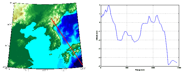
Matrix Map Values Along a Path

A common calculation for geographic matrix data is determining the values along a path. Examples include calculating terrain height along a straight section or along the path of a road. Use the mapprofile command to calulate regular matrix map values along a path. You can define the path and data by clicking on an existing map display, or by providing the command with a regular matrix map and vectors of waypoints. Similarly, the result can be displayed automatically in a new plot or returned as output arguments for furthur analysis or display.

Here is an example that shows the elevation profile along a straight line in the Korean elevation data.

Matrix Map Gradient, Slope, and Aspect

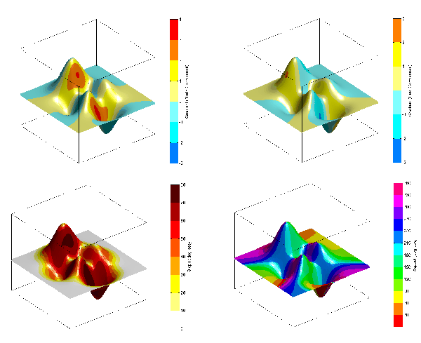
A map profile is often computed to find the slope along a path. A related calculation is the calculation of the slope at all points on a matrix. The gradientm command uses a finite-difference approach to compute the gradient of a regular or matrix map. The function returns the components of the gradient in the north and east directions, as well as the slope and aspect. The gradient components are the change in the map variable per meter of distance in the north and east directions. If the map contains elevations in meters, the aspect and slope are the angles of the surface normal clockwise from north and up from the horizontal. The angles are in units of degrees by default.

Here are the components of the gradient, slope, and aspect for a regular matrix map based on the MATLAB peaks matrix. The examples show the gradientm outputs as colors on a three-dimensional surface of elevation. The surfaces are shown with no vertical exaggeration:

• map = 500*peaks(100);
  maplegend = [ 1000 0 0];
  [aspect,slope,gradN,gradE] = gradientm(map,maplegend);
  

Visibility in Terrain

Regular matrix maps that contain elevation data can be used to answer questions about the mutual visibility of points. Is the line of sight from one point to another obscured by terrain? What area can be seen from a point, or the inverse question, what area can see that point?

The first question, on the line of sight between two points, can be answered with the los2 command. In the simplest calling form, los2 determines the visibility between two points on the surface of a digital elevation map. You can also specify the altitude of the observer and target points, as well as the datum with respect to which the altitudes are measured. For specialized applications, you can even control the actual and effective radius of the Earth, allowing use of the assumption frequently used in predicting radio wave propagation that the Earth has a radius 1/3 larger than the actual value.

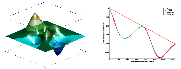
The following example shows the line of sight results between two points on the peaks regular matrix map. The calculation shows that the two points are mutually visible, but that the line of sight just barely clears an intervening peak. The los2 command also returns visibility results along the line of sight that can be used to understand why the answer is true or false:

• map = 500*peaks(100);
  maplegend = [ 1000 0 0];
  lat1 = -0.027; lon1 = 0.05; lat2 = -0.093; lon2 = 0.042;
    
  los2(map,maplegend,lat1,lon1,lat2,lon2,100)
  
  ans =
  
       1
  
  
     
  
  
  
  

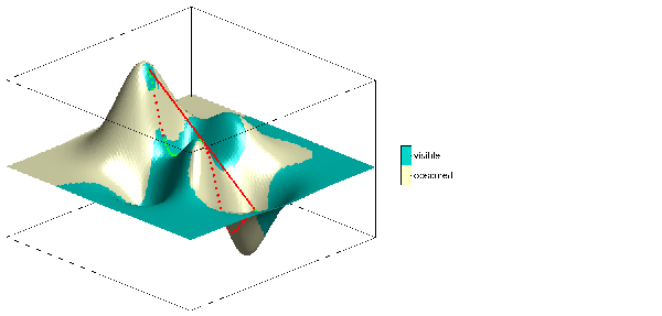
You can also compute the viewshed, a name derived from watershed, which is all of the areas that are visible from a particular point. The viewshed command can be thought of as performing the los2 line of sight calculation from one point on a digital elevation map to every other entry in the matrix. The viewshed command supports the same options as los2.

The following shows which parts of the peaks elevation map in the previous example are visible from the first point:

• [vismap,vismapleg] = viewshed(map,maplegend,lat1,lon1,100);
  
  
  

Working with Matrix Maps

General Matrix Maps