Financial Derivatives Toolbox

Self-Financing Hedges (hedgeslf)

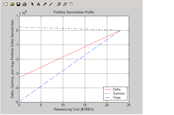
Figure 3-1 and Figure 3-2 indicate that there is no benefit to be gained because the funds available for hedging exceed $23,055.90, the point of maximum expense required to obtain simultaneous delta, gamma, and vega neutrality. You can also find this point of delta, gamma, and vega neutrality using hedgeslf.

• [Sens, Value1, Quantity] = hedgeslf(Sensitivities, Price,... 
  Holdings, FixedInd);
  
  Sens =
  
           -0.00
           -0.00
           -0.00
  
  Value1 =
  
        618.72
  
  Quantity =
  
          100.00
         -182.36
          -19.55
           80.00
            8.00
          -32.97
           40.00
           10.00
  

Similar to hedgeopt, hedgeslf returns the portfolio dollar sensitivities and instrument quantities (the rebalanced holdings). However, in contrast, the second output parameter of hedgeslf is the value of the rebalanced portfolio, from which you can calculate the rebalancing cost by subtraction.

• Value0 - Value1
  
  ans =
  
        23055.90
  

In our example, the portfolio is clearly not self-financing, so hedgeslf finds the best possible solution required to obtain zero sensitivities.

There is, in fact, a third calling syntax available for hedgeopt directly related to the results shown above for hedgeslf. Suppose, instead of directly specifying the funds available for rebalancing (the most money you are willing to spend), you want to simply specify the number of points along the cost frontier. This call to hedgeopt samples the cost frontier at 10 equally spaced points between the point of minimum cost (and potentially maximum exposure) and the point of minimum exposure (and maximum cost).

• [Sens, Cost, Quantity] = hedgeopt(Sensitivities, Price,... 
  Holdings, FixedInd, 10);
  
  Sens =
       -32784.46       2231.83     -49694.33
       -29141.74       1983.85     -44172.74
       -25499.02       1735.87     -38651.14
       -21856.30       1487.89     -33129.55
       -18213.59       1239.91     -27607.96
       -14570.87        991.93     -22086.37
       -10928.15        743.94     -16564.78
        -7285.43        495.96     -11043.18
        -3642.72        247.98      -5521.59
            0.00         -0.00          0.00
  
  Cost =
            0.00
         2561.77
         5123.53
         7685.30
        10247.07
        12808.83
        15370.60
        17932.37
        20494.14
        23055.90
  

Now plot this data.

• figure
  plot(Cost/1000, Sens(:,1), '-red')
  hold('on')
  plot(Cost/1000, Sens(:,2), '-.black')
  plot(Cost/1000, Sens(:,3), '--blue')
  grid
  xlabel('Rebalancing Cost ($1000''s)')
  ylabel('Delta, Gamma, and Vega Portfolio Dollar Sensitivities')
  title ('Portfolio Sensitivities Profile')
  legend('Delta', 'Gamma', 'Vega', 0)
  
  
  

Figure 3-3: Rebalancing Cost

In this calling form, hedgeopt calls hedgeslf internally to determine the maximum cost needed to minimize the portfolio sensitivities ($23,055.90), and evenly samples the cost frontier between $0 and $23,055.90.

Note that both hedgeopt and hedgeslf cast the optimization problem as a constrained linear least squares problem. Depending upon the instruments and constraints, neither function is guaranteed to converge to a solution. In some cases, the problem space may be unbounded, and additional instrument equality constraints, or user-specified constraints, may be necessary for convergence. See Hedging with Constrained Portfolios for additional information.

Hedging with hedgeopt

Specifying Constraints with ConSet