Curve Fitting Toolbox

smooth

Smooth the response data

Syntax

• yy = smooth(ydata)
  yy = smooth(ydata,span)
  yy = smooth(ydata,'method')
  yy = smooth(ydata,span,'method')
  yy = smooth(ydata,'sgolay',degree)
  yy = smooth(ydata,span,'sgolay',degree)
  yy = smooth(xdata,ydata,...)
  

Arguments

ydata	A column vector of response data.
span	The number of data points to include for each smooth calculation.
'method'	The smoothing method.
'sgolay'	Use Savitzky-Golay smoothing.
degree	The polynomial degree for the Savitzky-Golay method.
xdata	A column vector of predictor data.
yy	A vector of smoothed response data.

Description

yy = smooth(ydata) smooths the response data specified by ydata using the moving average method. The default number of data points in the average (the span) is five. yy is the smoothed response data. Note that you need not specify the predictor data if it is sorted and uniform.

yy = smooth(ydata,span) uses the number of data points specified by span in the moving average calculation. span must be odd.

yy = smooth(ydata,'method') smooths the response data using the method specified by method and the default span. The supported smoothing methods are given below. For the Savitzky-Golay method, the default polynomial degree is 2.

Method	Description
moving	Moving average filter.
lowess	Locally weighted scatter plot smooth using least squares linear polynomial fitting.
loess	Locally weighted scatter plot smooth using least squares quadratic polynomial fitting.
sgolay	Savitzky-Golay filter. Note that the algorithm used by the toolbox can accept nonuniform predictor data.
rlowess	Lowess smoothing that is resistant to outliers.
rloess	Loess smoothing that is resistant to outliers.

yy = smooth(ydata,span,'method') smooths data using the specified span and method. For the loess and lowess methods, you can specify span as a percentage of the total number of data points. In this case, span must be less than or equal to 1. For the moving average and Savitzky-Golay methods, span must be odd. If an even span is specified, it is reduced by 1.

yy = smooth(ydata,'sgolay',degree) uses the Savitzky-Golay method with polynomial degree specified by degree.

yy = smooth(ydata,span,'sgolay',degree) uses the number of data points specified by span in the Savitzky-Golay calculation. span must be odd and degree must be less than span.

yy = smooth(xdata,ydata,...) smooths the data specified by ydata and the associated predictor data, xdata. You should specify the predictor data when it is not uniformly spaced or it is not sorted. If xdata is not uniform and you do not specify method, lowess is used. If the smoothing method requires xdata to be sorted, the sorting occurs automatically.

Remarks

For the moving average and Savitzky-Golay methods, span must be odd. If an even span is specified, it is reduced by 1. If span is greater than the length of ydata, it is reduced to the length of ydata.

Use robust smoothing when you want to assign lower weight to outliers. The robust smoothing algorithm uses the 6MAD method, which assigns zero weight to data outside six mean absolute deviations.

Another way to generate a vector of smoothed response values is to fit your data using a smoothing spline. Refer to the fit function for more information.

Example

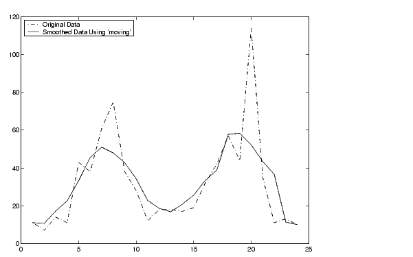
Suppose you want to smooth traffic count data with a moving average filter to see the average traffic flow over a 5-hour window (span is 5).

• load count.dat
  y = count(:,1);
  yy = smooth(y);
  

Plot the original data and the smoothed data.

• t = 1:length(y);
  plot(t,y,'r-.',t,yy,'b-')
  legend('Original Data','Smoothed Data Using ''moving''',2)
  
  
  
  

The first four elements of yy are given by

• yy(1) = y(1)
  yy(2) = (y(1)+y(2)+y(3))/3
  yy(3) = (y(1)+y(2)+y(3)+y(4)+y(5))/5
  yy(4) = (y(2)+y(3)+y(4)+y(5)+y(6))/5
  

Because of the way that the end points are treated, the result shown above differs from the result returned by the filter function described in Difference Equations and Filtering in the MATLAB documentation.

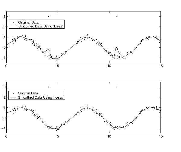
In this example, generate random data between 0 and 15, create a sine wave with noise, and add two outliers with the value 3.

• rand('state',2);
  x = 15*rand(150,1); 
  y = sin(x) + (rand(size(x))-0.5)*0.5;
  y(ceil(length(x)*rand(2,1))) = 3;
  

Smooth the data using the loess and rloess methods with the span specified as 10% of the data.

• yy1 = smooth(x,y,0.1,'loess');
  yy2 = smooth(x,y,0.1,'rloess');
  

Plot original data and the smoothed data.

• [xx,ind] = sort(x);
  subplot(2,1,1)
  plot(xx,y(ind),'r.',xx,yy1(ind),'k-')
  set(gca,'YLim',[-1.5 3.5])
  legend('Original Data','Smoothed Data Using ''loess''',2)
  subplot(2,1,2)
  plot(xx,y(ind),'r.',xx,yy2(ind),'k-')
  set(gca,'YLim',[-1.5 3.5])
  legend('Original Data','Smoothed Data Using ''rloess''',2)
  

Note how the outliers have less effect with the robust method.

See Also

fit, sort

set