Curve Fitting Toolbox

Fitting the Data

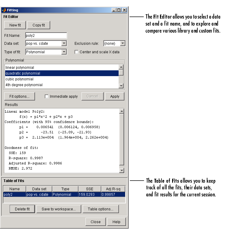
You fit data with the Fitting GUI. You open this GUI by clicking the Fitting button on the Curve Fitting Tool. The Fitting GUI consists of two parts: the Fit Editor and the Table of Fits. The Fit Editor allows you to

• Specify the fit name, the current data set, and the exclusion rule.
• Explore various fits to the current data set using a library or custom equation, a smoothing spline, or an interpolant.
• Override the default fit options such as the coefficient starting values.
• Compare fit results including the fitted coefficients and goodness of fit statistics.

The Table of Fits allows you to

• Keep track of all the fits and their data sets for the current session.
• Display a summary of the fit results.
• Save or delete the fit results.

The Data Fitting Procedure

For this example, begin by fitting the census data with a second degree polynomial. Then continue fitting the data using polynomial equations up to sixth degree, and a single-term exponential equation.

The data fitting procedure follows these general steps:

1. From the Fit Editor, click New Fit.

1. Note that this action always defaults to a linear polynomial fit type. You use New Fit at the beginning of your curve fitting session, and when you are exploring different fit types for a given data set.

2. Because the initial fit uses a second degree polynomial, select quadratic polynomial from the Polynomial list. Name the fit poly2.
3. Click the Apply button or select the Immediate apply check box. The library model, fitted coefficients, and goodness of fit statistics are displayed in the Results area.
4. Fit the additional library equations.

1. For fits of a given type (for example, polynomials), you should use Copy Fit instead of New Fit because copying a fit retains the current fit type state thereby requiring fewer steps than creating a new fit each time.

The Fitting GUI is shown below with the results of fitting the census data with a quadratic polynomial.

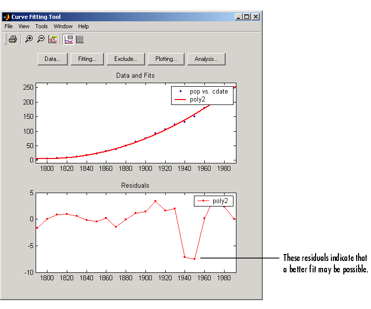
The data, fit, and residuals are shown below. You display the residuals as a line plot by selecting the menu item View->Residuals->Line plot from the Curve Fitting Tool.

The residuals indicate that a better fit may be possible. Therefore, you should continue fitting the census data following the procedure outlined in the beginning of this section.

The residuals from a good fit should look random with no apparent pattern. A pattern, such as a tendency for consecutive residuals to have the same sign, can be an indication that a better model exists.

When you fit higher degree polynomials, the Results area displays this warning:

• Equation is badly conditioned. Remove repeated data points
  or try centering and scaling.
  

The warning arises because the fitting procedure uses the cdate values as the basis for a matrix with very large values. The spread of the cdate values results in scaling problems. To address this problem, you can normalize the cdate data. Normalization is a process of scaling the predictor data to improve the accuracy of the subsequent numeric computations. A way to normalize cdate is to center it at zero mean and scale it to unit standard deviation.

• (cdate - mean(cdate))./std(cdate)
  

To normalize data with the Curve Fitting Tool, select the Center and scale X data check box.

Note    Because the predictor data changes after normalizing, the values of the fitted coefficients also change when compared to the original data. However, the functional form of the data and the resulting goodness of fit statistics do not change. Additionally, the data is displayed in the Curve Fitting Tool using the original scale.

Importing the Data

Determining the Best Fit