Curve Fitting Toolbox

Interpolants

Interpolation is a process for estimating values that lie between known data points. The supported interpolant methods are shown below.

Table 3-6: Interpolant Methods

Method	Description
Linear	Linear interpolation. This method fits a different linear polynomial between each pair of data points.
Nearest neighbor	Nearest neighbor interpolation. This method sets the value of an interpolated point to the value of the nearest data point. Therefore, this method does not generate any new data points.
Cubic spline	Cubic spline interpolation. This method fits a different cubic polynomial between each pair of data points.
Shape-preserving	Piecewise cubic Hermite interpolation (PCHIP). This method preserves monotonicity and the shape of the data.

The type of interpolant you should use depends on the characteristics of the data being fit, the required smoothness of the curve, speed considerations, postfit analysis requirements, and so on. The linear and nearest neighbor methods are fast, but the resulting curves are not very smooth. The cubic spline and shape-preserving methods are slower, but the resulting curves are often very smooth.

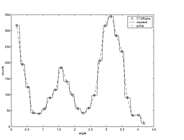
For example, the nuclear reaction data from the file carbon12alpha.mat is shown below with a nearest neighbor interpolant fit and a shape-preserving (PCHIP) interpolant fit. Clearly, the nearest neighbor interpolant does not follow the data as well as the shape-preserving interpolant. The difference between these two fits can be important if you are interpolating. However, if you want to integrate the data to get a sense of the total unormalized strength of the reaction, then both fits provide nearly identical answers for reasonable integration bin widths.

Note    Goodness of fit statistics, prediction bounds, and weights are not defined for interpolants. Additionally, the fit residuals are always zero (within computer precision) because interpolants pass through the data points.

Interpolants are defined as piecewise polynomials because the fitted curve is constructed from many "pieces." For cubic spline and PCHIP interpolation, each piece is described by four coefficients, which are calculated using a cubic (third-degree) polynomial. Refer to the spline function for more information about cubic spline interpolation. Refer to the pchip function for more information about shape-preserving interpolation, and for a comparison of the two methods.

Parametric polynomial fits result in a global fit where one set of fitted coefficients describes the entire data set. As a result, the fit can be erratic. Because piecewise polynomials always produce a smooth fit, they are more flexible than parametric polynomials and can be effectively used for a wider range of data sets.

Nonparametric Fitting

Smoothing Spline