Function Reference

pzmap

Compute the pole-zero map of an LTI model

Syntax

• pzmap(sys)
  pzmap(sys1,sys2,...,sysN)
  [p,z] = pzmap(sys)
  

Description

pzmap(sys) plots the pole-zero map of the continuous- or discrete-time LTI model sys. For SISO systems, pzmap plots the transfer function poles and zeros. For MIMO systems, it plots the system poles and transmission zeros. The poles are plotted as x's and the zeros are plotted as o's.

pzmap(sys1,sys2,...,sysN) plots the pole-zero map of several LTI models on a single figure. The LTI models can have different numbers of inputs and outputs and can be a mix of continuous and discrete systems.

When invoked with left-hand arguments,

• [p,z] = pzmap(sys)
  

returns the system poles and (transmission) zeros in the column vectors p and z. No plot is drawn on the screen.

You can use the functions sgrid or zgrid to plot lines of constant damping ratio and natural frequency in the - or -plane.

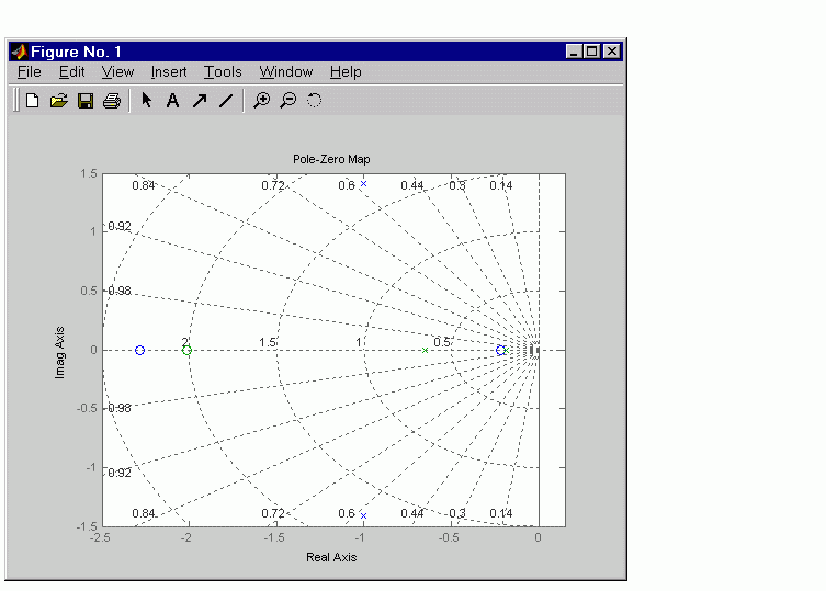
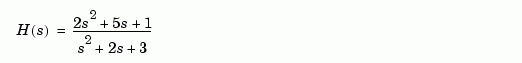
Example

Plot the poles and zeros of the continuous-time system.

• H = tf([2 5 1],[1 2 3]); sgrid
  pzmap(H)
  

Algorithm

pzmap uses a combination of pole and zero.

See Also
damp        Damping and natural frequency of system poles

esort, dsort  Sort system poles

pole        Compute system poles

rlocus      Root locus

sgrid, zgrid  Plot lines of constant damping and natural frequency

zero        Compute system (transmission) zeros

pole

reg