Communications Toolbox

Scatter Plots

A scatter plot of a signal shows the signal's value at a given decision point. In the best case, the decision point should be at the time when the eye of the signal's eye diagram is the most widely open.

To produce a scatter plot from a signal, use the scatterplot function. The signal can have different formats, as in the case of the eyediagram function. See the table Representing In-Phase and Quadrature Components of Signal for details.

Example: Scatter Plots

The code below is similar to the example from the section Example: Eye Diagrams. It produces a scatter plot from the received analog signal, instead of an eye diagram.

• % Define the M-ary number and sampling rates.
  M = 16; Fd = 1; Fs = 10;
  Pd = 200; % Number of points in the calculation
  msg_d = randint(Pd,1,M); % Random integers in the range [0,M-1]
  % Modulate using square constellation QASK method.
  msg_a = modmap(msg_d,Fd,Fs,'qask',M);
  % Assume the channel is equivalent to a raised cosine filter.
  rcv = rcosflt(msg_a,Fd,Fs);
  % Create the scatter plot of the received signal,
  % ignoring the first three and the last four symbols.
  N = Fs/Fd;
  rcv_a = rcv(3*N+1:end-4*N,:);
  h = scatterplot(rcv_a,N,0,'bx');
  

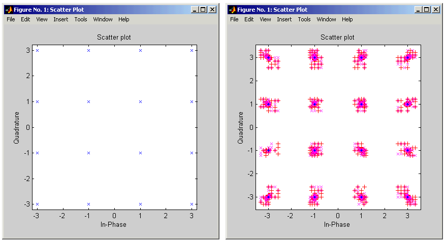
Varying the third parameter in the scatterplot command changes the offset. An offset of zero yields optimal results, shown on the left below.

The diagram on the right results from the commands below. The x's and +'s reflect two offsets that are not optimal because they are too late and too early, respectively. Notice that in the diagram, the dots are the actual constellation points, while the other symbols are perturbations of those points.

• hold on;
  scatterplot(rcv_a,N,N+1,'r+',h); % Plot +'s
  scatterplot(rcv_a,N,N-1,'mx',h); % Plot x's
  scatterplot(rcv_a,N,0,'b.',h); % Plot dots
  

Eye Diagrams

Source Coding