curl (MATLAB Functions)

Computes the curl and angular velocity of a vector field

Syntax

[curlx,curly,curlz,cav] = curl(X,Y,Z,U,V,W)
[curlx,curly,curlz,cav] = curl(U,V,W)
[curlz,cav]= curl(X,Y,U,V)
[curlz,cav]= curl(U,V)
[curlx,curly,curlz] = curl(...), [curlx,curly] = curl(...)
cav = curl(...)

Description

[curlx,curly,curlz,cav] = curl(X,Y,Z,U,V,W) computes the curl and angular velocity perpendicular to the flow (in radians per time unit) of a 3-D vector field U, V, W. The arrays X, Y, Z define the coordinates for U, V, W and must be monotonic and 3-D plaid (as if produced by meshgrid).

[curlx,curly,curlz,cav] = curl(U,V,W) assumes X, Y, and Z are determined by the expression:

```
[X Y Z] = meshgrid(1:n,1:m,1:p)
```

where [m,n,p] = size(U).

[curlz,cav]= curl(X,Y,U,V) computes the curl z-component and the angular velocity perpendicular to z (in radians per time unit) of a 2-D vector field U, V. The arrays X, Y define the coordinates for U, V and must be monotonic and 2-D plaid (as if produced by meshgrid).

[curlz,cav]= curl(U,V) assumes X and Y are determined by the expression:

```
[X Y] = meshgrid(1:n,1:m)
```

where [m,n] = size(U).

[curlx,curly,curlz] = curl(...), curlx,curly] = curl(...) returns only the curl.

cav = curl(...) returns only the curl angular velocity.

Examples

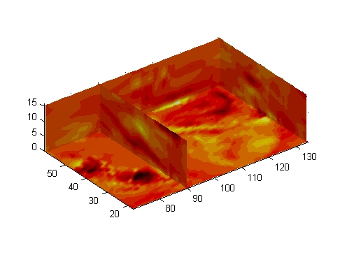
This example uses colored slice planes to display the curl angular velocity at specified locations in the vector field.

load wind
cav = curl(x,y,z,u,v,w);
slice(x,y,z,cav,[90 134],[59],[0]); 
shading interp
daspect([1 1 1]); axis tight
colormap hot(16)
camlight

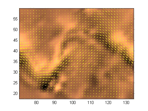
This example views the curl angular velocity in one plane of the volume and plots the velocity vectors (quiver) in the same plane.

load wind
k = 4;
x = x(:,:,k); y = y(:,:,k); u = u(:,:,k); v = v(:,:,k); 
cav = curl(x,y,u,v);
pcolor(x,y,cav); shading interp
hold on;
quiver(x,y,u,v,'y')
hold off
colormap copper

See Also

streamribbon, divergence

Volume Visualization for related functions

Displaying Curl with Stream Ribbons for another example

cumtrapz customverctrl